Bootstrapping Medians

Much of what I need to say about bootstrapping medians has already been said in the section on bootstrapping means. The procedures for bootstrapping almost any statistic follow a very predictable pattern, and I am not going to repeat much of that here. The only method that I have programmed as of the time of this original writing is "Lunneborg's" method.

Percentile Method

The percentile method applied to medians is essentially the same as that applied to means. We take our original sample of n observations, and sample from it, with replacement to create new samples. Each new sample contains n elements. We create B bootstrap samples, where B is a number of 1000 or more. These procedures draw at least 1000 bootstrap samples, and can draw as many as 50,000. The program runs so quickly that time is not really a concern for most purposes.

For each bootstrap sample we compute the sample median (denoted Med*), and when we have drawn all of our samples, these values of Med* represent the sampling distribution of the median. The program then sorts this sampling distribution for low to high (which can take a fair amount of time for very large values of B) and calculates the relevant percentiles. For our purposes here, these will be the 2.5th and 97.5th percentile, though generically these are the a/2 and 1-a/2 percentiles. For B = 1000, these will be the 25th and 975th order statistics (values from the ordered series). The percentile method would take these to be the upper and lower cutoffs for the 95% confidence interval.

Lunneborg's Method

As I said when I discussed bootstrapping limits on the mean, Lunneborg did not invent this approach (it is implicit in other sources), but his is a convenient name to assign.

When the sampling distribution is perfectly symmetric, the percentile method is quick, easy to comprehend, and accurate. But when the distribution isn't symmetric, better limits can be obtained by doing the same thing that we did with the mean. (I will use a = .05 and B = 1000 for a concrete example, assuming that you can make the obvious transition to other values.) First take the original sample, and calculate its median (denoted Med). Then do your resampling. Having drawn B bootstrap samples, we sort them as before from low to high.  We will take the distance from the original sample median to the 25th score, and label that "a." We take the distance from the 975th score to the original sample median and label that "b." Then the lower CI is Med - b, and the upper CI is Med + a. I am sure that you will think that I wrote that backw

Traditional Method

When we were working with the mean, we could fall back on the traditional method of creating confidence limits. This method computes . However, there are two important features of this approach. In the first place, it relies on the Student t distribution, which is based on an assumption of normality. Even if the population is not normal, the Central Limit Theorem tells us that the sampling distribution will be at least approximately normal, so we don't worry too much. We do not have a corresponding theorem for the median, and I don't know how quickly the sampling distribution approaches normal as n increases. Moreover, this formula requires that we estimate the standard error of the mean by taking the standard deviation of the sample and dividing by the square root of n. But we do not have a comparable formula when we are talking about the median, especially if the population is not normal. So the traditional method is out when it comes to the median.

Bootstrapped t Method

Just as we did with the mean, we can calculate a bootstrapped t estimate of the confidence limits for the median. However, we have to overcome at least two problems.

You should recall that for the mean we drew a bootstrapped sample, calculated the sample mean and standard deviation, converted that to a t* statistic by , and stored away the values of t*, which creates the sampling distribution of t*. Under ideal conditions this would simply reproduce Student's t distribution, and under less than ideal conditions this would reproduce something like, but more accurate than, Student's t distribution. The a/2 and 1-a/2 cutoffs give us the t values we need for the traditional approach.

However, we have a problem. We could, and will, substitute Med* and Med for and to calculate t, but what do we use for ? This is our estimate of the standard error, but it only works for the mean. It is not the standard error of the median.  To get the standard error of the median, we have to have the empirical standard deviation of a bunch of medians. In other words, at this point in our calculations we have to come to a full stop, draw a bunch of new bootstrap samples, using our current bootstrap sample as if it were the original sample, calculate the standard deviation of that bunch of sample medians, then calculate t, and go on with drawing bootstrap sample number 2. (The concept of dividing (Med* - Med) by its standard error is known as Studentizing, and it is an important step. In other words, we need to do bootstrapping within bootstrapping. That is a lot of work, but computers never need to sleep or rest, so it is not impossible. 

Let B represent the number of bootstrap samples we calculate in the outer loop, and let b represent the number of bootstrap samples we draw based on each outer bootstrap samples. Thus we will draw B*b samples in all. Efron works in terms of B being a number on the order of 1000, while b is a number on the order of 50. There is nothing sacred about these values, but they should give you the general idea. 

One more step. From the subsamples taken above, we will get B values of t*, from which we will find the a/2 and 1-a/2 cutoffs. We use those as we have in the traditional method. But we need one more thing--we need the standard error of the median that corresponds to the standard error of the mean in the traditional formula. We can obtain an estimate of that by taking the medians of our B samples, and simply calculating the standard deviation of that distribution. Then our confidence limits become. This is analogous to what we did with the mean.

I have discussed this approach with respect to the median, but you could use it with respect to a wide array of statistics. The nice thing is that we don't need to know a formula for the standard error we seek--we just go out and estimate it by brute force.

Diagram of the bootstrapped t method:

Original Sample:  2   2   3   4   5   5   5   6  7   9  --> Med  

Sample 1:    2   2   2   5   6   6   6   7   7   9 --> Med1*

                                Subsample 1a:        2   2   5   5   5   5   6   6   7   9 --> Med1a

                                Subsample 1b:        2   5   5   5   6   7   7   7   7   9 --> Med1b

                                Subsample 1c:        2   5   5   6   6   6   7   7   9   9  --> Med1c

                    Sample 2:    3   3   3   5   5   5   6   6   6    9  --> Med2*

                                Subsample 2a:        3   3   5   5   6   6   6   9   9   9  -->  Med2a

                                Subsample 2b:        3   3   3   3   5   5   5   6   6   9  --> Med2b

                                Subsample 2c         3   3   5   5   5   5   5   6   6   9  -->  Med2c

                    Med = median of original sample--around which we will build our interval

Med1*, Med2*, etc. = Outer set of bootstrapped medians, which will give us standard error of the median.

Med1a, Med1b, Med1c, etc--inner set of bootstrapped medians, which will be used to calculate t*₁. Similarly for Med2a, Med2b, and Med2c. These sets will generate the estimate of the standard error of Med*1, Med*2, etc.

Although I have discussed the bootstrapped t method in some detail, it is not implemented in Resampling.exe.

Better intervals

I could say the same things here that I said for confidence limits on the mean, with respect for corrections for bias and acceleration. I will not repeat that here, but the translation should be straightforward--though the calculations are not.

Reaction time example

The Resampling.exe program calculates a confidence interval on the median using the bootstrapped t approach. We can illustrate the result of this method using an example that I have used elsewhere. This is based on a study by Sternberg (1966), in which he asked subjects to view a set of digits for a brief time (measured in milliseconds) and then see a test digit. They were required to press one key if the test digit had been present in the comparison digits, and press a different key if it had not. I will use the data from the condition in which 5 comparison digits were first presented, and the test stimulus actually was one of those digits.

The distribution of reaction times is somewhat skewed. Notice that it has a range of about 60 milliseconds, with a mean of about 65 milliseconds (the median was 62). We would expect a positive skew because of the nature of the task.

If we were calculating 95% confidence limits on the mean, SPSS could tell us that those limits were 61.01 and 68.19. However, SPSS cannot give us limits on the median

If we use our program to calculate confidence limits on the median, we obtain the following results.

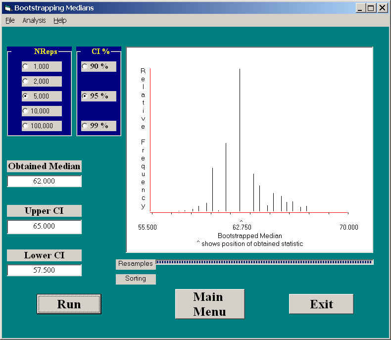
Notice that these limits are somewhat narrower (57.5 and 65.0) and that they are slightly asymmetric around the sample median. The number of different values of the medians in bootstrapped samples were rather limited, but that is because the median must either be one of the obtained values, or the average of two of them. Note also the slight positive skewness of the sampling distribution of the median. The median is not as well behaved as the mean relative to the central limit theorem, which does not apply to medians.